library("tibble")
library("dplyr")
library("tidyr")
library("broom")
library("ggplot2")
library("ggrepel")In this brief post, we will take a look at what happens if we mix data science and music… Should be good… For this post to make sense, you’ll need to know a bit of musical theory and a bit of data science - Enjoy!
First, let us start off by loading some packages:
Then, we will one-hot encode the major scale of each key by denoting a given tone 1 if it is in the scale and a 0 otherwise:
major_scales <- tribble(
  ~key, ~C, ~`C#`, ~D, ~Eb, ~E, ~F, ~`F#`, ~G, ~`G#`, ~A, ~Bb, ~B,
  "C",    1,   0,    1,  0,   1,  1,   0,    1,   0,    1,  0,   1,
  "C#",   1,   1,    0,  1,   0,  1,   1,    0,   1,    0,  1,   0,
  "D",    0,   1,    1,  0,   1,  0,   1,    1,   0,    1,  0,   1,
  "Eb",   1,   0,    1,  1,   0,  1,   0,    1,   1,    0,  1,   0,
  "E",    0,   1,    0,  1,   1,  0,   1,    0,   1,    1,  0,   1,
  "F",    1,   0,    1,  0,   1,  1,   0,    1,   0,    1,  1,   0,
  "F#",   0,   1,    0,  1,   0,  1,   1,    0,   1,    0,  1,   1,
  "G",    1,   0,    1,  0,   1,  0,   1,    1,   0,    1,  0,   1,
  "G#",   1,   1,    0,  1,   0,  1,   0,    1,   1,    0,  1,   0,
  "A",    0,   1,    1,  0,   1,  0,   1,    0,   1,    1,  0,   1,
  "Bb",   1,   0,    1,  1,   0,  1,   0,    1,   0,    1,  1,   0,
  "B",    0,   1,    0,  1,   1,  0,   1,    0,   1,    0,  1,   1
)
Then we will perform a Principal Component Analysis of the data:
scales_pca <- major_scales %>%
  column_to_rownames("key") %>%
  prcomp %>%
  tidy %>%
  rename(key = row) %>%
  filter(PC %>% between(1, 2)) %>%
  pivot_wider(id_cols = key,
              names_from = PC,
              values_from = value) %>%
  rename(PC1 = `1`,
         PC2 = `2`)
Finally, we will visualise the data using the first two principal components:
scales_pca %>%
  ggplot(aes(x = PC1,
             y = PC2,
             label = key)) +
  geom_label() +
  coord_fixed() +
  theme_minimal()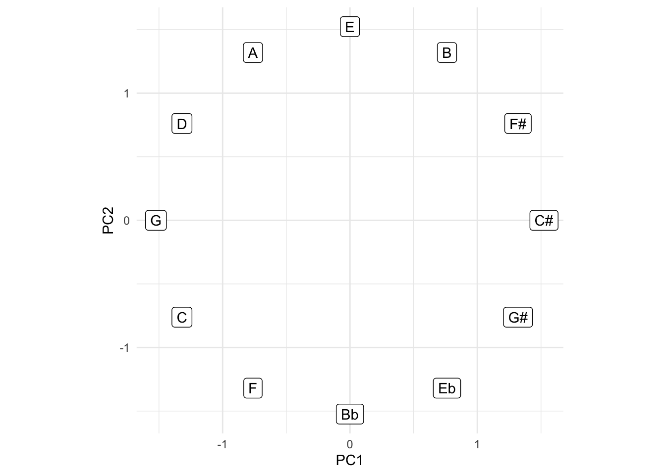
Looks familiar? But what happens if we add minor as well?
minor_scales <- tribble(
  ~key, ~C, ~`C#`, ~D, ~Eb, ~E, ~F, ~`F#`, ~G, ~`G#`, ~A, ~Bb, ~B,
  "Cm",   1,   0,    1,  1,   0,  1,   0,    1,   1,    0,  1,   0,
  "C#m",  0,   1,    0,  1,   1,  0,   1,    0,   1,    1,  0,   1,
  "Dm",   1,   0,    1,  0,   1,  1,   0,    1,   0,    1,  1,   0,
  "Ebm",  0,   1,    0,  1,   0,  1,   1,    0,   1,    0,  1,   1,
  "Em",   1,   0,    1,  0,   1,  0,   1,    1,   0,    1,  0,   1,
  "Fm",   1,   1,    0,  1,   0,  1,   0,    1,   1,    0,  1,   0,
  "F#m",  0,   1,    1,  0,   1,  0,   1,    0,   1,    1,  0,   1,
  "Gm",   1,   0,    1,  1,   0,  1,   0,    1,   0,    1,  1,   0,
  "G#m",  0,   1,    0,  1,   1,  0,   1,    0,   1,    0,  1,   1,
  "Am",   1,   0,    1,  0,   1,  1,   0,    1,   0,    1,  0,   1,
  "Bbm",  1,   1,    0,  1,   0,  1,   1,    0,   1,    0,  1,   0,
  "Bm",   0,   1,    1,  0,   1,  0,   1,    1,   0,    1,  0,   1,
)
…and again, we perform a PCA:
scales_pca <- major_scales %>%
  bind_rows(minor_scales) %>%
  column_to_rownames("key") %>%
  prcomp %>%
  tidy %>%
  rename(key = row) %>%
  filter(PC %>% between(1, 2)) %>%
  pivot_wider(id_cols = key,
              names_from = PC,
              values_from = value) %>%
  rename(PC1 = `1`,
         PC2 = `2`)
…and visualise using ggrepel to avoid overlapping labels:
scales_pca %>%
  ggplot(aes(x = PC1,
             y = PC2,
             label = key)) +
  geom_label_repel() +
  geom_point() +
  coord_fixed() +
  theme_minimal()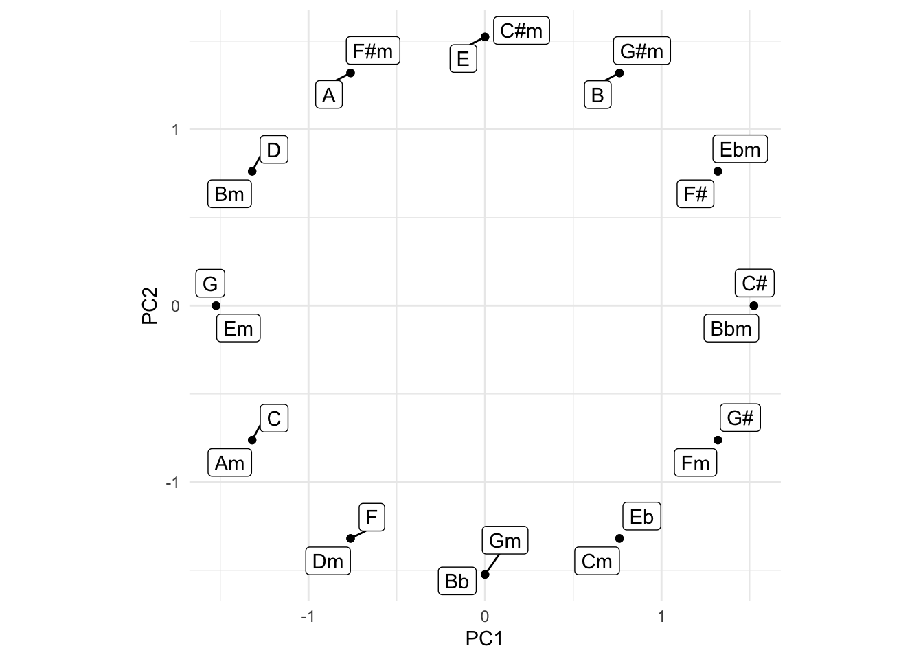
…and there you have it - If you do a PCA on one-hot encoded major and minor scales, you get the circle of fifths!